2 Data

2.1 Description

As we are studying crimes at NYC parks and potential reasons, we collected three datasets: park crimes, unemployment, and mobility data.

First, we collected crime data in NYC from NYPD official websites focused on crime statistics. The link for the data is NYPD Crime Statistics. The data covers quarters from 2014 to 2023. The data for each quarter shows features like numbers of crimes, park sizes, and boroughs. The data format is an excel file for each quarter that we downloaded onto our local drives and imported into R. All of the downloaded data is available in this Github folder for ease of reference and reproducibility. Once the data was imported, we cleaned and merged data for all quarters. For our study, we explored total number of different types of crimes, park size categories, and boroughs.

Second, we collected unemployment data from U.S. Bureau of Labor Statistics official website focused on the NYC area. The link of data is NYC Unemployment Statistics. Additionally, BLS Data Finder offered on this website is able to search unemployment data for NYC. We downloaded an excel file with all of the data from 2013-2023 onto our local drive and imported into R for our project. The file we imported is available here for ease of reference and reproducibility. Monthly unemployment data is available from 2013 to 2023. Columns include the year, month, and annual average unemployment in wide format.

Last, we looked at high level mobility data from Google Community Mobility Reports. The link for data is Mobility Data. Daily data showing movement trends in places such as parks is available during the Covid-19 period. A few restrictions on this data include: it is only available from February 2020 to February 2022, and the data must be scraped from the published reports. To use this data, one must use a third party source that has scraped data into a csv file or complete the scrape themselves. We chose to use an exiting scrape, and the link for data is this GitHub Repo. Though the dataset includes other locations (such as grocery stores), and other regions (different states in the US), we focused only on parks and NYC. We imported this data directly from github as a csv file for our analysis. The values provided show deviations from the baseline, which is set as the 5-week period Jan 3–Feb 6, 2020. We also note that any correlations generated from this data are at risk of containing a confounding variable since the data is only available during the pandemic period.

2.2 Research Plan

We plan to use NYC crimes data to track how the frequency of different types of crimes has changed across time and in different boroughs. We will then use unemployment data to glean any additional insights or correlations that may exist. Lastly, we will derive any impacts of park visit frequency from February 2020-February 2022. A few different ideas for analysis are included below:

Time series analysis for crimes data. We will conduct time series analysis to look into components including long term trends, seasonality (systematic, calendar related movements), and irregularity (unsystematic, short term fluctuations). In addition to overall crime trends, we will further analyze how specific types of crimes (murder, rape, etc.) vary over time.
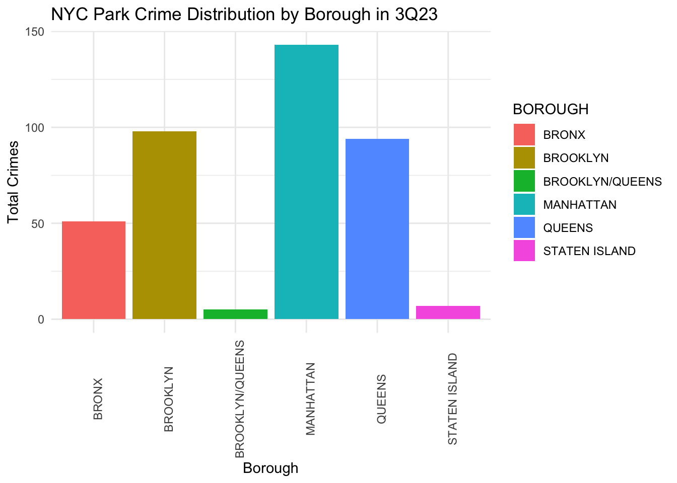
Heatmaps and bar charts for crimes data. We will illustrate crimes data in heatmaps based on boroughs and periods to find time and regional differences. We will use bar charts to show the total number of crimes in each borough, allowing for easy comparison across regions.
Relationship between crimes and employment rate. We will look into trends for total number of crimes and unemployment rates. We will first demonstrate these two variables in line graphs to see the trends over time. We will then compare the trend lines for crime rates and unemployment rates to see if they are similar.
Relationship between crimes and mobility data. For February 2020 to February 2022, we will look into the number of crimes and park attendance levels, investigating whether visitor flow affects crimes by analyzing trend lines.

2.3 Missing value analysis

2.3.1 Crimes Data

First, we examine the crimes dataset. As a sample, we will pull data for 3Q23 for a high level overview. After determining data cleans, we will merge data for multiple quarters. We can see that there are few missing values in our data. We can just delete the records with missing values.

Code

library(readxl)
nyc_park_crime_stats_q3_2023 <- read_excel("~/Desktop/crime_data/nyc-park-crime-stats-q3-2023.xlsx") #read data

# show part of data
head(nyc_park_crime_stats_q3_2023)

# A tibble: 6 × 12
  3rd QTR PARK CRIME REP…¹ ...2  ...3  ...4  ...5  ...6  ...7  ...8  ...9  ...10
  <chr>                    <chr> <chr> <chr> <chr> <chr> <chr> <chr> <chr> <chr>
1 SEVEN MAJOR COMPLAINTS   <NA>  <NA>  <NA>  <NA>  <NA>  <NA>  <NA>  <NA>  <NA> 
2 Report covering the per… <NA>  <NA>  <NA>  <NA>  <NA>  <NA>  <NA>  <NA>  <NA> 
3 PARK                     BORO… SIZE… CATE… MURD… RAPE  ROBB… FELO… BURG… GRAN…
4 CORONA HEALTH SANCTUARY  QUEE… 0.101 PLAY… 0     0     0     0     0     0    
5 LT. FEDERICO NARVAEZ TO… BROO… 0.125 PLAY… 0     0     0     0     0     0    
6 SOBEL PLAYGROUND         BROO… 0.135 PLAY… 0     0     0     0     0     0    
# ℹ abbreviated name: ¹`3rd QTR PARK CRIME REPORT`
# ℹ 2 more variables: ...11 <chr>, ...12 <chr>

We can see that there are a few extra rows of data at the top and row 3 needs to be the header.

Code

colnames(nyc_park_crime_stats_q3_2023) = nyc_park_crime_stats_q3_2023[3,] #set row 3 as header
nyc_park_crime_stats_q3_2023 = nyc_park_crime_stats_q3_2023[-c(1,2,3), ] #remove first 3 rows of data
head(nyc_park_crime_stats_q3_2023) #new data column names

# A tibble: 6 × 12
  PARK     BOROUGH `SIZE (ACRES)` CATEGORY MURDER RAPE  ROBBERY `FELONY ASSAULT`
  <chr>    <chr>   <chr>          <chr>    <chr>  <chr> <chr>   <chr>           
1 CORONA … QUEENS  0.101          PLAYGRO… 0      0     0       0               
2 LT. FED… BROOKL… 0.125          PLAYGRO… 0      0     0       0               
3 SOBEL P… BROOKL… 0.135          PLAYGRO… 0      0     0       0               
4 BILL BO… MANHAT… 0.172          BASKETB… 0      0     0       0               
5 WILLIAM… QUEENS  0.230          PLAYGRO… 0      0     1       2               
6 SUNSHIN… MANHAT… 0.240          PLAYGRO… 0      0     0       0               
# ℹ 4 more variables: BURGLARY <chr>, `GRAND LARCENY` <chr>,
#   `GRAND LARCENY OF MOTOR VEHICLE` <chr>, TOTAL <chr>

Here, we show the features of crimes data: park, borough, park size, number of crimes by type of crime.

Code

# examine whether thre are missing values
colSums(is.na(nyc_park_crime_stats_q3_2023))

                          PARK                        BOROUGH 
                             0                              1 
                  SIZE (ACRES)                       CATEGORY 
                             1                              1 
                        MURDER                           RAPE 
                             0                              0 
                       ROBBERY                 FELONY ASSAULT 
                             0                              0 
                      BURGLARY                  GRAND LARCENY 
                             0                              0 
GRAND LARCENY OF MOTOR VEHICLE                          TOTAL 
                             0                              0

Here, we can see there are only some missing values in each column, which are negligible. Therefore we just delete the records with missing values.

Code

nyc_park_crime_stats_q3_2023_clean <- na.omit(nyc_park_crime_stats_q3_2023)
head(nyc_park_crime_stats_q3_2023_clean)

# A tibble: 6 × 12
  PARK     BOROUGH `SIZE (ACRES)` CATEGORY MURDER RAPE  ROBBERY `FELONY ASSAULT`
  <chr>    <chr>   <chr>          <chr>    <chr>  <chr> <chr>   <chr>           
1 CORONA … QUEENS  0.101          PLAYGRO… 0      0     0       0               
2 LT. FED… BROOKL… 0.125          PLAYGRO… 0      0     0       0               
3 SOBEL P… BROOKL… 0.135          PLAYGRO… 0      0     0       0               
4 BILL BO… MANHAT… 0.172          BASKETB… 0      0     0       0               
5 WILLIAM… QUEENS  0.230          PLAYGRO… 0      0     1       2               
6 SUNSHIN… MANHAT… 0.240          PLAYGRO… 0      0     0       0               
# ℹ 4 more variables: BURGLARY <chr>, `GRAND LARCENY` <chr>,
#   `GRAND LARCENY OF MOTOR VEHICLE` <chr>, TOTAL <chr>

To visualize the crimes by borough, we first compute the total crimes.

Code

library(dplyr)
nyc_park_crime_stats_q3_2023_clean <- nyc_park_crime_stats_q3_2023_clean %>%
  mutate_at(vars(TOTAL), as.numeric)

# compute total crimes for boroughs
borough_crime_totals <- nyc_park_crime_stats_q3_2023_clean %>%
  group_by(BOROUGH) %>%
  summarize(Total_Crimes = sum(TOTAL, na.rm = TRUE))

print(borough_crime_totals)

# A tibble: 6 × 2
  BOROUGH         Total_Crimes
  <chr>                  <dbl>
1 BRONX                     51
2 BROOKLYN                  98
3 BROOKLYN/QUEENS            5
4 MANHATTAN                143
5 QUEENS                    94
6 STATEN ISLAND              7

Then we use bar chart to show the results.

Code

library(ggplot2)
borough_data = as.data.frame(borough_crime_totals)

ggplot(borough_data, aes(x = BOROUGH, y = Total_Crimes, fill = BOROUGH)) +
    geom_bar(stat="identity") +
    theme_minimal() +
    labs(title="NYC Park Crime Distribution by Borough in 3Q23", x="Borough", y="Total Crimes") +
    theme(axis.text.x = element_text(angle = 90))

2.3.2 Unemployment Rate Data

Then, we examine the dataset for unemployment rates.

Code

unemployment_rate <- read_excel("~/Desktop/unemployment_rate.xlsx") #read data
print(unemployment_rate)

# A tibble: 11 × 14
    Year   Jan   Feb   Mar   Apr   May   Jun   Jul   Aug   Sep   Oct   Nov   Dec
   <dbl> <dbl> <dbl> <dbl> <dbl> <dbl> <dbl> <dbl> <dbl> <dbl> <dbl> <dbl> <dbl>
 1  2013   9.1   9.1   9     9     8.9   8.9   8.9   8.9   8.7   8.6   8.4   8.2
 2  2014   8     7.8   7.6   7.5   7.3   7.1   6.9   6.8   6.6   6.5   6.4   6.3
 3  2015   6.2   6.1   6     5.9   5.7   5.6   5.4   5.2   5.2   5.1   5.2   5.2
 4  2016   5.2   5.2   5.2   5.1   5.1   5.2   5.2   5.3   5.2   5.2   5     4.9
 5  2017   4.7   4.6   4.5   4.5   4.5   4.6   4.6   4.6   4.5   4.5   4.4   4.3
 6  2018   4.3   4.2   4.2   4.1   4.1   4     4     4     4.1   4.2   4.3   4.3
 7  2019   4.3   4.2   4.1   4     3.9   3.8   3.8   3.8   3.8   3.8   3.9   4  
 8  2020   4.1   4.3   4.5  12.7  21.4  17.1  16.5  14.8  14.3  13.2  12.9  12.6
 9  2021  12.3  11.9  11.4  11.1  10.4  10.5   9.8   9.6   8.8   8.5   8.1   8  
10  2022   7.6   6.9   6.3   5.9   5.5   5.2   4.9   4.6   4.9   5.2   5.2   5.1
11  2023   5.3   5.4   5.3   5.4   5.3   5.4   5.3   5.3   5.3   5.4  NA    NA  
# ℹ 1 more variable: Avg <lgl>

It’s obvious that the missing values are average unemployment rates for each year and the last two months in 2023. For the average rates, we can directly compute the average rates based on monthly rates.

Code

unemployment_rate$Avg <- rowMeans(unemployment_rate[, 2:13], na.rm = TRUE)

As for missing values for the last two months in 2023, it’s reasonable because there is no data available yet for months in the future. We can just ignore the missing values here.

Code

print(unemployment_rate)

# A tibble: 11 × 14
    Year   Jan   Feb   Mar   Apr   May   Jun   Jul   Aug   Sep   Oct   Nov   Dec
   <dbl> <dbl> <dbl> <dbl> <dbl> <dbl> <dbl> <dbl> <dbl> <dbl> <dbl> <dbl> <dbl>
 1  2013   9.1   9.1   9     9     8.9   8.9   8.9   8.9   8.7   8.6   8.4   8.2
 2  2014   8     7.8   7.6   7.5   7.3   7.1   6.9   6.8   6.6   6.5   6.4   6.3
 3  2015   6.2   6.1   6     5.9   5.7   5.6   5.4   5.2   5.2   5.1   5.2   5.2
 4  2016   5.2   5.2   5.2   5.1   5.1   5.2   5.2   5.3   5.2   5.2   5     4.9
 5  2017   4.7   4.6   4.5   4.5   4.5   4.6   4.6   4.6   4.5   4.5   4.4   4.3
 6  2018   4.3   4.2   4.2   4.1   4.1   4     4     4     4.1   4.2   4.3   4.3
 7  2019   4.3   4.2   4.1   4     3.9   3.8   3.8   3.8   3.8   3.8   3.9   4  
 8  2020   4.1   4.3   4.5  12.7  21.4  17.1  16.5  14.8  14.3  13.2  12.9  12.6
 9  2021  12.3  11.9  11.4  11.1  10.4  10.5   9.8   9.6   8.8   8.5   8.1   8  
10  2022   7.6   6.9   6.3   5.9   5.5   5.2   4.9   4.6   4.9   5.2   5.2   5.1
11  2023   5.3   5.4   5.3   5.4   5.3   5.4   5.3   5.3   5.3   5.4  NA    NA  
# ℹ 1 more variable: Avg <dbl>

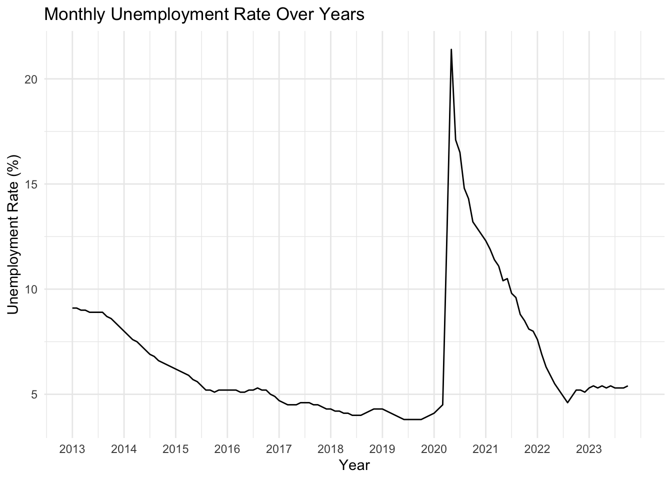
The following line graph is a time series visualization showing the variation in unemployment rates for each month across different years. There are no gaps in this plot, verifying no missing values in the dataset.

Code

library(ggplot2)
library(tidyr)
library(dplyr)

unemployment_long <- unemployment_rate %>%
  pivot_longer(cols = Jan:Dec, names_to = "Month", values_to = "UnemploymentRate") %>%
  mutate(Month = match(Month, month.abb))

ggplot(unemployment_long, aes(x = Year + (Month-1)/12, y = UnemploymentRate)) +
  geom_line() +
  scale_x_continuous(breaks = unique(unemployment_long$Year)) +
  labs(title = "Monthly Unemployment Rate Over Years",
       x = "Year",
       y = "Unemployment Rate (%)") +
  theme_minimal()

2.3.3 Mobility Data

We examine the mobility dataset. We only focus on the feature: parks_percent_change_from_baseline.

Code

#import data

data = read.csv('https://raw.githubusercontent.com/ActiveConclusion/COVID19_mobility/master/google_reports/mobility_report_US.csv')

# Step 2: Filter for New York Data and Parks
nyc_data <- data %>%
  filter(state == "New York") %>%
  select(county, date, parks)
head(nyc_data)

  county       date parks
1  Total 2020-02-15    -2
2  Total 2020-02-16    13
3  Total 2020-02-17    23
4  Total 2020-02-18    -4
5  Total 2020-02-19    11
6  Total 2020-02-20     0

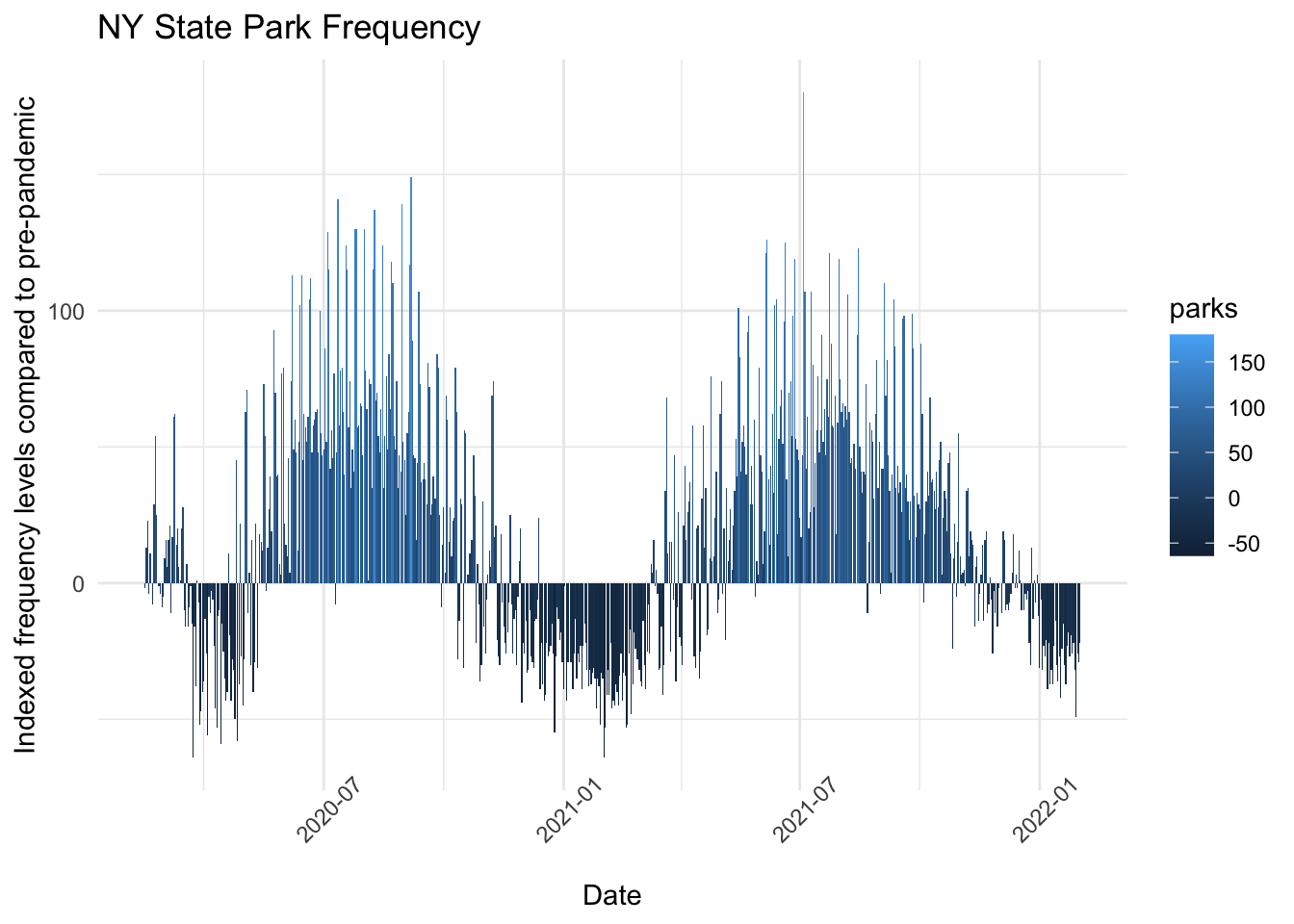
This data shows changes in park visit frequency relative to pre-pandemic levels. For example, in the table above, we can see that total New York park visits were down 2 points on February 15th 2020 and up 13 points on February 16th 2020.

Code

# Step 3: Visualization for total NY park frequency
ny_summary = nyc_data %>%
  filter(county == "Total")
ny_summary$date = as.Date(ny_summary$date)

ggplot(ny_summary, aes(x = date, y = parks, fill = parks)) +
    geom_bar(stat = "identity") +
    theme_minimal() +
    labs(title = "NY State Park Frequency", x = "Date", y = "Indexed frequency levels compared to pre-pandemic") +
    theme(axis.text.x = element_text(angle = 45))

Since the Mobility data is defined by counties and our NYC crimes data is defined by borough, we can filter for counties that encompass in the 5 NYC boroughs.

Code

selected_regions <- nyc_data %>%
  filter(county %in% c("Bronx County", "Kings County", "Queens County", 
                             "New York County", "Richmond County"))

# Replace borough names
selected_regions <- selected_regions %>%
  mutate(county = case_when(
    county == "Bronx County" ~ "BRONX",
    county == "Kings County" ~ "BROOKLYN",
    county == "Queens County" ~ "QUEENS",
    county == "New York County" ~ "MANHATTAN",
    county == "Richmond County" ~ "STATEN ISLAND",
    TRUE ~ county
  ))

Next we test whether there are missing values in selected boroughs.

Code

na_count_parks_percent_change <- sum(is.na(selected_regions$parks_percent_change_from_baseline))

print(na_count_parks_percent_change)

[1] 0

The result shows that the dataset is complete without missing values. Then we can draw the summarized bar chart based on selected boroughs.

Code

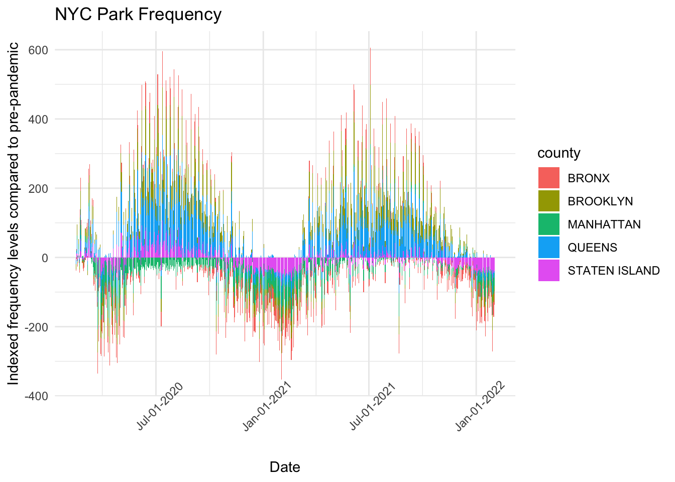
library(scales)
selected_regions$date = as.Date(selected_regions$date)
ggplot(selected_regions, aes(fill=county, y=parks, x=date)) + 
    geom_bar(position="stack", stat="identity") +
    theme_minimal() +
    labs(title = "NYC Park Frequency", x = "Date", y = "Indexed frequency levels compared to pre-pandemic") +
    theme(axis.text.x = element_text(angle = 45)) +
    scale_x_date(date_labels = "%b-%d-%Y")

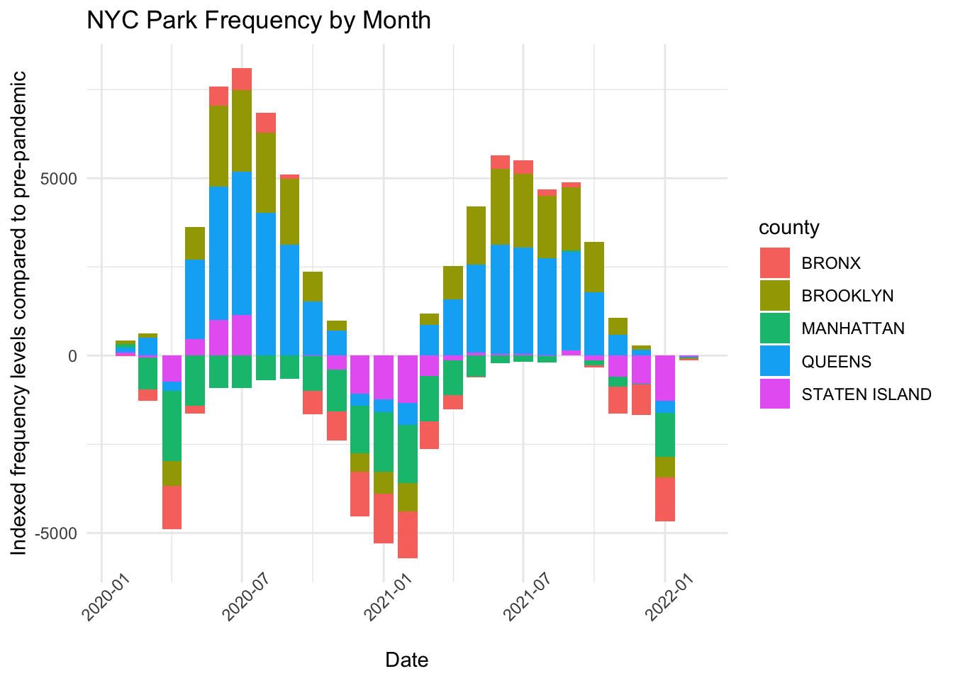
Since the data is tough to read in detail, we can summarize it by each month of data collected

Code

selected_regions$date = as.Date(selected_regions$date)
monthly_values = selected_regions %>% 
    group_by(month = lubridate::floor_date(date, 'month'), county) %>%
    summarize(sum = sum(parks))

ggplot(monthly_values, aes(fill=county, y=sum, x=month)) + 
    geom_bar(position="stack", stat="identity") +
    theme_minimal() +
    labs(title = "NYC Park Frequency by Month", x = "Date", y = "Indexed frequency levels compared to pre-pandemic") +
    theme(axis.text.x = element_text(angle = 45))